Theory

Nonlinear optical susceptibility

The SHG phenomenon of a NLO material arises from how the electrons of the material respond to the oscillating electric field \(\mathbf{E}\) of light, which can be described by the electric polarization \(\mathbf{P}\) expressed as,

\(\mathbf{P} = \mathbf{P}^{(0)} + \mathbf{P}^{(1)} + \mathbf{P}^{\left( 2 \right)} + \ldots,\) (1)

where\(\ \mathbf{P}^{(0)}\), \(\mathbf{P}^{(1)}\) and \(\mathbf{P}^{(2)}\) are the zero-, first- and second-order polarization, respectively. \(\mathbf{P}^{(0)}\) is independent of \(\mathbf{E}\), with components \(P_{o}^{(0)}\) (o = x, y, z). With \(\epsilon_{0}\) as the electric permittivity of the vacuum and using the Einstein summation convention, the \(i\)^th components of \(\mathbf{P}^{(1)}\) and \(\mathbf{P}^{(2)}\) (in the domain of frequency\((\omega\)) can be written as

\(P_{o}^{(1)}\left( \omega \right) = \epsilon_{0}\chi_{\text{op}}^{\left( 1 \right)}\left( \omega \right)E_{p}\left( \omega \right),\) (2)

\(P_{o}^{(2)}\left( \omega \right) = \epsilon_{0}\chi_{\text{opq}}^{\left( 2 \right)}\left( \omega \right)E_{p}\left( \omega_{1} \right)E_{q}\left( \omega_{2} \right).\) (3)

In Eq. 2, \(\omega\) refers to the frequency of the pump light as well as that of the response signal. The linear electric susceptibility \(\mathbf{\chi}^{(1)}\) is a second-rank tensor, while the non- linear electric susceptibility tensor \(\mathbf{\chi}^{(2)}\) is a third-rank tensor. In Eq. 3, \(\omega_{i},(i = 1,\ 2\)) the frequencies of the pump light and \(\omega = \omega_{1} + \omega_{2}\) represents the frequency of the signal light. \(\mathbf{\chi}^{(1)}\) and \(\mathbf{\chi}^{(2)}\) are the first- and second-order functional derivatives of \(\mathbf{P}\) with respect to \(\mathbf{E}\), while the zero-order (or spontaneous) polarization \(\mathbf{P}^{(0)}\) has no dependence on the electric field. In fact, it is due to this reason that the static dipole moment is not explicitly related to the SHG response as shown below,

\(\chi^{\left( 2 \right)} = \frac{\delta^{2}\mathbf{P}^{(2)}\lbrack\mathbf{E},\ \ \mathbf{E}\rbrack}{\delta\mathbf{E}^{\mathbf{2}}}\) (4)

which represents a second-order functional derivative with respect to the electrical field of a light, The NLO tensors \(\mathbf{\chi}^{(n)}\) are calculated using quantum perturbation theory, while we confine the emphasis on the ART, which maps \(\mathbf{\chi}^{(2)}\) onto the constituent atoms of a NLO crystal material.

The partial response functional (PRF) method

For a general response function\(\text{F}\left( x \right)\), the variable \(x\) covers the range of –∞<\(x\)<+∞. If we suppress other variables of \(F\left( x \right)\ \) for simplicity, the PRF covering the contribution from the region of \(x\)₀≤\(x\)<+∞ can be defined as

\(\text{ζ}\left( x_{0},F \right) = \int_{- \infty}^{+ \infty}{H\left( x - x_{0} \right)F\left( x \right)\text{dx}}\) (5)

Where \(H\left( x - x_{0} \right)\) is the Heaviside step function (i.e., 0 for \(x\) < \(x\)₀, and 1 for \(x\) ≥ \(x\)₀). Note that \(x\)₀ is the variable of the functional. The PRF covering the contribution from the region of –∞<\(x\)≤\(x\)₀ can be defined as

\(\text{ζ}\left( x_{0},F \right) = \int_{- \infty}^{+ \infty}{\left\{ 1 - H\left( x - x_{0} \right) \right\} F\left( x \right)\text{dx}}\) (6)

The derivative functional \(\text{δζ}\left( x_{0},F \right)\ \)with respect to \(x\)₀ provides the value of the response function at \(x\)₀, namely, \(\text{∓}\)F(\(x\)₀), where the minus and positive signs correspond to the cases of Eq. 5 and 6, respectively.

\(\text{δζ}\left( x_{0},F \right)\ \equiv \ \frac{\text{dζ}\left( x_{0},F \right)}{dx_{0}}\)

\(= \text{∓}\int_{- \infty}^{+ \infty}{\delta\left( x - x_{0} \right)F\left( x \right)\text{dx} = \text{∓}F\left( x_{0} \right)}\) (7)

PRF for SHG susceptibility

When the variable \(x\) is a continuous number, such as the energy E, with the E_B of Fig. 1 acting as the \(x\)₀, the domain of the variable E can be regarded as –∞<E<+∞. For each SHG coefficient \(\chi_{\text{opq}}^{\left( 2 \right)}\) taken as the response function \(F\left( E \right)\), we determine the PRF \(\zeta{(E}_{B},\chi_{\text{opq}}^{\left( 2 \right)})\) contributed from a partial region of the VBs by using Eq. 5 (denoted as \(\zeta_{V}{(E}_{B})\ \)in Fig. 1b), which arises from a partial region of CBs by using Eq. 6 (denoted as \(\zeta_{C}{(E}_{B})\) in Fig. 1c). It should be noted that \(\zeta_{V}{(E}_{B})\) [\(\zeta_{C}{(E}_{B})\)] becomes the total response when E_B reaches E_min (E_max).

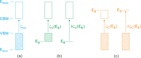
Fig. 1. Concepts of the PRFs for SHG responses: (a) The total response \(\mathbf{\zeta}_{\mathbf{\text{tot}}}\). (b) The partial responses associated with the VBs. \(\mathbf{\zeta}_{\mathbf{V}}\mathbf{(E}_{\mathbf{B}}\mathbf{)}\) refers to the contribution from all states of the VBs lying above E_B to all CBs, and \(\mathbf{\delta}\mathbf{\zeta}_{\mathbf{V}}\mathbf{(E}_{\mathbf{B}}\mathbf{)}\) to that only from the E_B level to all CBs. (c) The partial responses associated with the CBs. \(\mathbf{\zeta}_{\mathbf{C}}\mathbf{(E}_{\mathbf{B}}\mathbf{)}\) refers to the contribution from all states of the VBs to all states of the CBs up to E_B, and \(\mathbf{\delta}\mathbf{\zeta}_{\mathbf{C}}\mathbf{(E}_{\mathbf{B}}\mathbf{)}\) to that from all VBs only to the E_B of the CBs

The variable \(x\) can also be an integer such as the band index I, which runs from 1 for the lowest-lying energy band and increases with increasing the band energy E, reaching N_tot (i.e., the total number of bands in a given system) for the highest-lying energy band. In this case, the domain of I is 1≤I≤N_tot, and a specific band I_s within the VBs or that within the CBs plays the role of \(x\)₀. Therefore, the PRFs can also be discussed in terms of the band index using the specific band I_s, leading to the corresponding functionals \(\zeta_{V}{(I}_{s})\) and \(\zeta_{C}{(I}_{s})\) for VBs and CBs, respectively.

Considering both the specific band energy E_B and the band index I_s, there are four derivative PRFs denoted as \(\text{δζ}_{V}(I_{s})\), \(\text{δζ}_{C}\left( I_{s} \right)\), \(\text{δζ}_{V}(E_{B})\), and \(\text{δζ}_{C}\left( E_{B} \right)\), which are associated with the PRFs \(\zeta_{V}(I_{s})\), \(\zeta_{C}\left( I_{s} \right)\), \(\zeta_{V}(E_{B})\), and \(\zeta_{C}\left( E_{B} \right)\) correspondingly. \(\text{δζ}_{V}(I_{s})\) provides the contribution of the valence band \(I_{s}\). Similarly, \(\text{δζ}_{C}\left( I_{s} \right)\) shows the contribution of the conduction band \(I_{s}\). Thus, it is possible to calculate the contribution that a specific atom \(\tau\) makes to the SHG coefficient from the band state \(I_{s}\) by using its tight-binding atomic orbital representation provided by various first principles DFT codes such as VASP, etc.^[27].

\(\delta\zeta_{V}{(E}_{B}) = - \frac{d\zeta_{V}{(E}_{B})}{\text{dE}_{B}}\) (8)

\(\delta\zeta_{C}{(E}_{B}) = \frac{d\zeta_{C}{(E}_{B})}{\text{dE}_{B}}\) (9)

Atom response theory (ART) analyses

To evaluate the individual atom contributions to the components of a SHG tensor, \(\mathbf{\chi}^{(2)}\), it is computationally more convenient to use the PRFs in terms of the band index I_B, \(\zeta(I_{B})\)^[12], with increasing energy, \(E_{B}\). Here, \(\zeta_{V}(I_{B})\) and \(\zeta_{C}(I_{B})\) are denoted as \(_{}^{\text{VB}}\zeta_{j}\) and \(_{}^{\text{CB}}\zeta_{j}\), respectively, with I_B replaced by a subscript j. Suppose that a specific atom \(\tau\) has \(L\) atomic orbitals with a coefficient \(_{}^{\text{VB}}C_{\text{Lτ}}^{\overrightarrow{k}j}\) in the valence band \(j\) at a wave vector\(\ \overrightarrow{k}\). The total contribution \(_{}^{\text{VB}}A_{\tau}^{}\) that an atom \(\tau\) makes to the SHG coefficient from all the valence bands \(\text{j}\) is written as

\(_{}^{\text{VB}}A_{\tau} = \frac{\Omega}{\left( 2\pi \right)^{3}}\int_{}^{}{d\overrightarrow{k} \bullet \sum_{L,j}^{}{_{}^{\text{VB}}\zeta_{j}}}\left|_{}^{\text{VB}}C_{\text{Lτ}}^{\overrightarrow{k}j} \right|^{2}\) (10)

where \(\Omega\) is the unit cell volume and \(_{}^{\text{VB}}\zeta_{j}\) is the corresponding PRFs in terms of the band index j. Similarly, the total contribution \(_{}^{\text{CB}}A_{\tau}^{}\) that an atom \(\tau\) makes to the SHG coefficient from all the conduction bands \(j\) is written as

\(_{}^{\text{CB}}A_{\tau} = \frac{\Omega}{\left( 2\pi \right)^{3}}\int_{}^{}{d\overrightarrow{k} \bullet \sum_{L,j}^{}{_{}^{\text{CB}}\zeta_{j}}}\left|_{}^{\text{CB}}C_{\text{Lτ}}^{\overrightarrow{k}j} \right|^{2}\) (11)

in which we assumed that the atom has \(L\) atomic orbitals with coefficient \(_{}^{\text{CB}}C_{\text{Lτ}}^{\overrightarrow{k}j}\) in the conduction band \(j\) at a wave vector \(\overrightarrow{k}\). To calculate the actual contribution of each constituent atom in a unit cell to the total SHG response, one needs to consider the signs of \(_{}^{\text{VB}}\zeta_{j}\) and \(_{}^{\text{CB}}\zeta_{j}\). The total contribution, \(A_{\tau}\), is given by

\(A_{\tau} = \frac{\left(_{}^{\text{VB}}A_{\tau}^{}\ +_{}^{\text{\ CB}}A_{\tau}^{} \right)}{2}\) (12)

where the factor of 1/2 is applied to remove the double-counting of each excitation. From Eqs. 10～12, the total contribution as well as the orbital contribution of individual atoms to any components of the SHG tensors for a given compound can be quantitatively obtained.

General principles for partitioning an extended structure and its physical property

For crystal materials, the functional motif (unit or group) has been used in the literature to describe the “materials gene” determining a specific material property. Currently, structural groups based on chemical stability are widely used to refer to a functional motif. However, theoretically, the partitioning method of an extended structure depends closely on its physical properties. Due to the lack of a structural partition based on physical properties, it is impossible to obtain the correct functional motif controlling a specific physical property of materials. Here, we present our newly proposed general concepts and principles for partitioning an extended structure at the atomic scale. The extended structures are composed of covalent and/or ionic bonds. Suppose that each atom of an extended structure is represented by a geometric point, and each covalent or ionic bond between them by a line specific to its bonding type. Mathematically, then, an extended structure is a connected set, to be denoted as \(\mathcal{X}\), which cannot be partitioned in a rigorous sense. The energy of an extended system \(\mathcal{X}\) can be written as

\(H = \sum_{i}^{}{H_{i} +}\sum_{i < j}^{}H_{\text{ij}}\) (13)

where \(H_{i}\) is an onsite energy for each point, \(\text{and }H_{\text{ij}}\) for each bond between points \(i\) and \(j\). For any two points in \(\mathcal{X,}\) there is always a path connecting them, i.e., \(H_{\text{ij}} \neq 0\) for all bonds on the path. Eq. 13 is essentially a tight-binding (TB) Hamiltonian, which results from averaging out all degrees of freedom of electrons in a Hamiltonian at electron scale. The typical Hamiltonian for a system of N nonrelativistic electrons and M nuclei is given by

\(H = \sum_{i = 1}^{N}\frac{\mathbf{p}_{i}^{2}}{2m} + \sum_{i < j}^{}\frac{e^{2}}{\left| \mathbf{r}_{i} - \mathbf{r}_{j} \right|} - \sum_{i,j = 1}^{N,M}\frac{{Z_{j}e}^{2}}{\left| \mathbf{r}_{i} - \mathbf{R}_{j} \right|}\)

\(+ \sum_{i < j}^{}\frac{{Z_{i}Z_{j}e}^{2}}{\left| \mathbf{R}_{i} - \mathbf{R}_{j} \right|} + \sum_{i = 1}^{M}\frac{\mathbf{P}_{i}^{2}}{2M_{i}}\) (14)

where \(\mathbf{P}_{i}\), \(M_{i,}\) and \(Z_{i}\) represent the momentum, mass, and the effective charge of the i^th nucleus, respectively, while \(\mathbf{p}_{i}\) and \(m\) are the momentum and mass of the i^th electron, respectively. In general, Eq. 14 is solved by adopting the Born-Oppenheimer approximation, which leaves the nuclei coordinates {\(\mathbf{R}_{j}\)} as the fixed parameters of the electronic structure problem. In solving the resulting electronic Schrödinger equation, one introduces further approximations, such as the DFT method, etc. How to deduce the \(H_{i}\) and \(H_{\text{ij}}\) terms of the TB Hamiltonian from the first-principles DFT calculations have been discussed by Sutton et al. The energy partitioning scheme of Eq. 13 is very useful in understanding the chemical bonding of a compound. For example, each \(H_{\text{ij}}\) (\(i \neq j\)) term is the kernel of the COHP bond indicator. To partition an extended structure, it is necessary to set some \(H_{\text{ij}}\) to zero, namely, to cut some bonds in a physical system. Hence, a thumb rule for partitioning an extended structure is to choose the weakest bonds, i.e., those with small \(|H_{\text{ij}}|\) values, to cut. The physical property, \(\mathbb{P}\), of an extended crystal is calculated at the electronic scale, i.e., \(\mathbb{P}\mathbb{= \ P}\left( x_{1},x_{2},\cdots \right),\) where \(x_{i}\ \)= (\(\mathbf{r}_{i},\sigma_{i}\)) denotes the position and spin coordinates of the i^th electron. In discussing the structure-property correlation of an extended system, it is necessary to calculate the property \(\mathcal{P}\) defined at the atomic scale, i.e., \(\mathcal{P = \ P}\)(\(\mathbf{R}_{1},\mathbf{R}_{2},\cdots\)), where \(\mathbf{R}_{i}\) refers to i^th nuclear position. Both \(\mathbb{P}\) and \(\mathcal{P}\) have similar structures, namely,

\(\mathbb{P =}\sum_{i}^{}{f(x_{i};{\{\mathbf{R}}_{l}\})} + \sum_{i < j}^{}{g(x_{i},x_{j};{\{\mathbf{R}}_{l}\})}\) (15)

\(\mathcal{P =}\sum_{i}^{}{\mathcal{F}\left( \mathbf{R}_{i} \right)} + \sum_{i < j}^{}{\mathcal{G}\left( \mathbf{R}_{i},\mathbf{R}_{j} \right)}\ \) (16)

The information from \(\mathcal{P}\) is more valuable for chemists and material scientists because they can help derive the functional motifs for a property \(\mathbb{P}\), thus providing clues to the search for new materials. The rigorous transformation from Eq. 15 to Eq. 16 presents an unsolved scale change problem. In practice, numerical methods with approximations such as the tight-binding approximation etc. are often used to map \(\mathbb{P}\) onto \(\mathcal{P}\).

In principle, the inter-atomic contribution as shown in Eq. 16 can be integrated into the atomic contribution by summing over all atoms paired with a specific atom, e.g., the one at \(\mathbf{R}_{i}\), as shown below,

\(\mathcal{P =}\sum_{i}^{}{\mathcal{F'(}\mathbf{R}_{i})}\) (17)

with

\(\mathcal{F}^{'}\left( \mathbf{R}_{i} \right)\mathcal{= F}\left( \mathbf{R}_{i} \right) + \frac{1}{2}\sum_{j \neq i}^{}{\mathcal{G(}\mathbf{R}_{i},\mathbf{R}_{j})}\) (18)

where the factor 1/2 accounts for double-counting of interatomic contributions when Eq. 16 is used to calculate 𝒫. Eq. 16 is mathematically equivalent to Eq. 15 and is useful for describing very local properties, such as incoherent scattering phenomena as well as NLO or other optical properties. However, in this partitioning, the role of the structure becomes implicit.

To find the functional motif of a material concerning its specific property\(\ \mathcal{P}\), we use Eq. 17 and assign the contributions of the center/interior atoms of a group solely to the group. In principle, one can choose those atoms with a large weight of \(\mathcal{P}\) as the interior atoms of a group, although this way of partitioning is property-dependent. Our strategy is to leave the functional motif undetermined at the beginning; after the individual atomic contributions, \(\mathcal{F}^{'}\left( \mathbf{R}_{i} \right)\), are obtained, one can decide the motif by comparing the total contributions of different groups. The groups can be chosen as the polyhedra built according to the following procedures; 1) Construct the polyhedra of nonmetal cations covalently bonded to their nearest neighbours. 2) Construct the polyhedra centred around metal cations with their neighbours. 3) Each polyhedron contains only one cation at the centre. 4) Any two polyhedra may share a vertex, an edge, or a face, but should not interpenetrate.