
ARTATOP Examples
This tutorial demonstrates how to obtain:
- Linear Optical Properties
- Nonlinear Optical Properties
- Atomic Contributions to SHG response
Example 1: Optical Properties of LiIO₃ (Based on VASP OPTIC Output)
This example aims to briefly introduce the program's parameters and the overall workflow. Computational costs have been simplified for clarity, and users should test the convergence of related results themselves.
Building upon the static (ground-state) calculation, new parameters must be added to the INCAR file to obtain the necessary electronic structure and position matrix elements for subsequent ARTATOP calculations. The key parameters that need to be specified in the INCAR are as follows (for reference)
SYSTEM = LiIO3
ENCUT= 600 eV
ISMEAR = -5
NELMDL = -5
NELMIN = 4
EDIFF = 0.00001
NELM = 60
IBRION = -1
POTIM = 0.4
LORBIT=10
KSPACING=0.2
KGAMMA=.TRUE.
NBANDS = 168
LOPTICS = .TRUE.
CSHIFT = 0.1
NEDOS = 3000
NPAR = 1
Note: To achieve converged optical properties, the value of the NBANDS parameter must be increased to at least three times the number used in the self-consistent field calculation.
Additionally, NPAR = 1 must be set to ensure the output of the OPTIC file.
1.1 Linear Optical Properties Calculation
In the directory containing the VASP optical property calculation results, create an input file named input_lin to specify the parameters for the linear optical property calculation. Simultaneously, create an output directory named out_lin to store the results.
The parameters in the input_lin file should be set as follows:
Input File (input_lin)
LO 77
$dft_src lvasp=T $end
$opc maxomega = 16  domega = 0.01167  scissor=1.7929  ecutmin = 0.03  smear = 0.03  $end
Run Command
artatop < input_lin > re_lin
ARTATOP will commence the calculation and output the linear optical properties of the material. The runtime information is logged in the file re_lin.
The numerical results are saved in the previously created out_lin directory. Each component is stored in a separate file named in the format lin_component.dat. The naming convention for all nine components is as follows: Output files (out_lin/) include:
lin_xx.dat  lin_xy.dat  lin_xz.dat
lin_yx.dat  lin_yy.dat  lin_yz.dat
lin_zx.dat  lin_zy.dat  lin_zz.dat
Each output file contains the energy-dependent linear optical properties, specifically: Dielectric function ε: Imaginary part (ε₂), Real part (ε₁), and Absolute value (|ε|) Extinction coefficient (κ) Refractive index (n) Reflectivity (R) Absorption coefficient (α)
A data excerpt from the result file lin_xx.dat is presented below:
# the data is generated at 10:50:23 on 2025/11/23
# calculated the x,x component of dielectric function
# smear:    0.030000eV
# scissor:    0.832700eV
# energy window:   96.368026eV

#   Energy(eV)         Im(eps)         Re(eps)         abs(eps)
    0.000000E+00    2.019569E-18    4.385258E+00    4.385258E+00
    1.167000E-02    4.536555E-05    4.385267E+00    4.385267E+00
    2.334000E-02    9.073307E-05    4.385293E+00    4.385293E+00
    3.501000E-02    1.361046E-04    4.385338E+00    4.385338E+00
    4.668000E-02    1.814820E-04    4.385399E+00    4.385399E+00
    …
#   Energy(eV)          kappa          Refractive index
    0.000000E+00      0.000000E+00      2.094101E+00
    1.167000E-02      1.083174E-05      2.094103E+00
    2.334000E-02      2.166388E-05      2.094109E+00
    3.501000E-02      3.249684E-05      2.094120E+00
    4.668000E-02      4.333102E-05      2.094134E+00
    …
#   Energy(eV)      Reflectivity from vacuum, at normal incidence
    0.000000E+00    1.250391E-01
    1.167000E-02    1.250404E-01
    2.334000E-02    1.250423E-01
    3.501000E-02    1.250448E-01
    4.668000E-02    1.250480E-01
    …
#   Energy(eV)      Absorption coeff
    0.000000E+00    0.000000E+00
    1.167000E-02    1.281187E+00
    2.334000E-02    5.124845E+00
    3.501000E-02    1.153126E+01
    4.668000E-02    2.050092E+01
    …
Based on the data above, the energy-dependent linear optical properties of LiIO₃ can be obtained, as shown in the following figure:
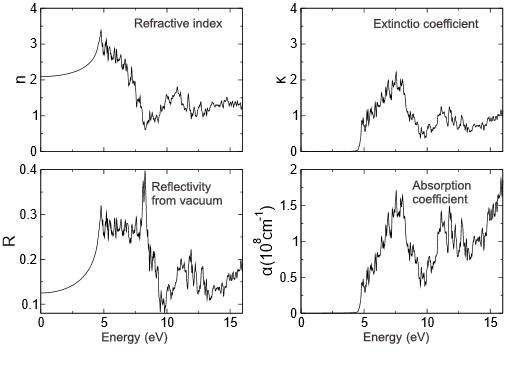
Fig. 1. The refractive index (n), reflectivity (R), extinction coefficient (κ), and absorption coefficient (α) of LiIO₃ as functions of incident photon energy.
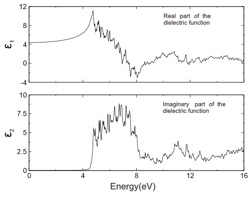
Fig. 2. Real (ε₁) and imaginary (ε₂) parts of the dielectric function for LiIO₃ as functions of incident photon energy.
1.2 SHG Coefficient Calculation
To calculate the second-harmonic generation coefficients, create an input file named input_nlin within the VASP optical property calculation directory to specify the relevant computational parameters. Additionally, establish a folder named out_nonlin for storing the output results.
The parameters in the input_nlin file should be set as follows:
Input File (input_nlin)
NO 777
$dft_src lvasp=T $end
$opc maxomega = 16 domega = 0.01167 scissor=1.7929 ecutmin = 0.03  smear = 0.03  $end
Run Command
artatop < input_nlin > re_nlin
The calculation results are stored in the created out_nonlin directory, with files named in the
format nonlin_component.dat. The naming convention for all 27 tensor components is as follows: out_nonlin/ directory with format "nonlin_ Component .dat".
The calculation results are stored in the created out_nonlin directory, with files named in the format nonlin_component.dat. The naming convention for all 27 tensor components is as follows:
nonlin_xxx.dat nonlin_xyz.dat nonlin_yxy.dat nonlin_yzx.dat
nonlin_zxz.dat nonlin_zzy.dat nonlin_xxy.dat nonlin_xzx.dat
nonlin_yxz.dat nonlin_yzy.dat nonlin_zyx.dat nonlin_zzz.dat
nonlin_xxz.dat nonlin_xzy.dat nonlin_yyx.dat nonlin_yzz.dat
nonlin_zyy.dat nonlin_xyx.dat nonlin_xzz.dat nonlin_yyy.dat
nonlin_zxx.dat nonlin_zyz.dat nonlin_xyy.dat nonlin_yxx.dat
nonlin_yyz.dat nonlin_zxy.dat nonlin_zzx.dat
nonlin_component.dat files contain the following data for the SHG susceptibility: the real part, imaginary part, and magnitude of the total SHG coefficient, as well as the real part, imaginary part, and magnitude of its interband and intraband contributions. Additionally, the files include the individual interband transition term (χ), intraband transition term (η), and the modulation term (σ) representing the intraband modulation of interband transitions.
A data excerpt from the result file nonlin_xyz.dat is presented below:
# the data is generated at 09:57:30 on 2025/11/23
# calculated the z,x,x component of second harmonic generation
# smear: 0.030000 eV
# scissor: 0.832700 eV
# ecutmin: 0.030000 eV
# energy window: 96.368026 eV
# Energy Tot-Im Chi(-2w,w,w) Tot-Re Chi(-2w,w,w) |TotChi(-2w,w,w)|
# eV 10^-7 esu 10^-7 esu 10^-7 esu
0.000000E+00 -2.671353E-02 -2.239006E-01 2.254886E-01
1.167000E-02 -2.680699E-02 -2.247326E-01 2.263258E-01
2.334000E-02 -2.690109E-02 -2.255720E-01 2.271704E-01
3.501000E-02 -2.699584E-02 -2.264187E-01 2.280223E-01
4.668000E-02 -2.709125E-02 -2.272728E-01 2.288818E-01
...
Based on the data above, the energy-dependent second-order nonlinear optical properties of ZnS can be obtained, as shown in the following figure:
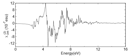
Fig. 3. SHG coefficient \(\chi_{zxx}^{(2)}\) of LiIO\(_3\) as a function of incident photon energy.
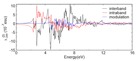
Fig. 4. The interband term, intraband term, and interband-to-intraband modulation term of \(\chi_{zxx}^{(2)}\) for LiIO\(_3\) as functions of incident photon energy.
1.3 Individual Atom Contributions to SHG Using ARTATOP
To analyze the individual atomic contributions to the SHG coefficient using Atomic Response Theory (ART), create an input file named input_art within the VASP optical property calculation directory. Additionally, establish a folder named out_nonlin to store the calculation results.
The parameters in the input_art file should be configured as follows:
Input File (input_art)
AR 411
$dft_src lvasp=T $end
$opc maxomega = 0.0 domega = 0.01167 scissor=1.7929 ecutmin = 0.03  smear = 0.03  $end
Run Command
artatop < input_art > re_art
The output results are stored in the created out_nonlin directory. All seven generated files are listed as follows:
  arp_dshg_zxx.txt    arp_dshg-vb_zxx.txt    arp_dshg-cb_zxx.txt
  arp_nonlin.txt      arp_shg_val_zxx.txt    arp_shg_con_zxx.txt
  arp_nshg_zxx.txt
The contents of the output files will be briefly introduced below. First, the data contained in arp_nshg_zxx.txt includes:
# iband   Im Chi(-2w,w,w)   Re Chi(-2w,w,w)
   1     -2.671353E-02   -2.239006E-01
   2     -2.720657E-02   -2.252791E-01
   3     -2.693385E-02   -2.256414E-01
   4     -2.890958E-02   -2.407479E-01
   5     -2.803404E-02   -2.486163E-01
   6     -2.823418E-02   -2.521489E-01
Using the data from arp_nshg_xyz.txt and arp_dshg_xxx.txt, graphical representations of the partial response functions (PRF) within any desired energy range can be generated:
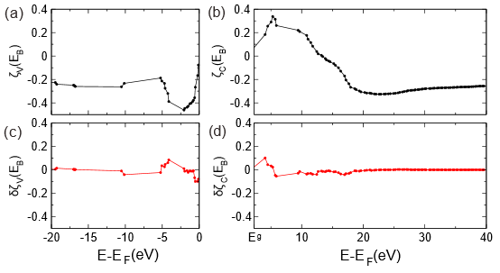
Fig. 5. PRF for \(\chi_{123}^{(2)}\) of LiIO\(_3\). (a) \(\zeta_V(E_B)\) vs. \(E_B\), (b) \(\zeta_C(E_B)\) vs. \(E_B\), (c) \(\delta\zeta_V(E_B)\) vs. \(E_B\), and (d) \(\delta\zeta_C(E_B)\) vs. \(E_B\).
The arp_nonlin.txt file contains the contribution of each atomic orbital to the SHG coefficient. This file includes data for 30 orbitals (for LiIO3), with the orbital order corresponding to the atomic and orbital sequence in the PROCAR file. Based on these results, the percentage contribution of each atom to the total SHG coefficient can be calculated, as shown in the following table:
| elements | s | p | d | Total |
|---|---|---|---|---|
| Li | 0.354 | 9.969 | 0.000 | 10.323 |
| I | 9.099 | -26.182 | 27.199 | 10116 |
| O | -6.240 | 85.801 | 0.000 | 79.561 |
To obtain the contributions of atomic orbitals in the valence (VB) and conduction bands (CB), the data from arp_shg_val_zxx.txt and arp_shg_con_zxx.txt should be used. This enables the calculation of the percentage contribution from the valence band part and conduction band part of each atom to the total second-harmonic generation coefficient, as presented in the following table:
| Atom | VB | CB | ||||
|---|---|---|---|---|---|---|
| s | p | d | s | p | d | |
| Li | -1.994 | 0.173 | 0.000 | 2.348 | 9.795 | 0.000 |
| I | 7.772 | -21.529 | 2.204 | 1.327 | -4.652 | 24.995 |
| O | -6.626 | 74.086 | 0.000 | 0.385 | 11.74 | 0.000 |
Example 2: GaAs (Based on ABINIT Optical Module Output)
Optical Property Calculation with ABINIT
The DDK output information for GaAs is obtained through ABINIT calculations. Below is a sample optic.abi input file (for reference) required for calculating optical properties with ABINIT:
GaAs sample input file
ndtset 6
#First dataset
  nband1 28
  nstep1 1000
  kptopt1 1
  nbdbuf1 0
 prtden1 1   getden1 0   getwfk1 0    # Usual file handling data
toldfe1 2.0d-8

#Second dataset
  iscf2 -2
  nstep2 1000
  kptopt2  1
  getwfk2  1   getden2 1

#Third dataset
  iscf3 -2
  nstep3 1000
  getwfk3  2
  getden3 1

  prtwant3  2
  w90iniprj3 2

  #Fourth dataset
  iscf4 -3
  nstep4  1  nline4  0  prtwf4  3

  nqpt4  1    qpt4  0.0d0 0.0d0 0.0d0
  rfdir4  1 0 0
  rfelfd4  2
  #Fifth dataset
  iscf5 -3
  nstep5  1  nline5  0  prtwf5  3

  nqpt5  1    qpt5  0.0d0 0.0d0 0.0d0
  rfdir5  0 1 0
  rfelfd5  2

#Sixth dataset
  iscf6 -3
  nstep6  1  nline6  0  prtwf6  3

  nqpt6  1    qpt6  0.0d0 0.0d0 0.0d0
  rfdir6  0 0 1
  rfelfd6  2

# Data common to datasets 2-6
  nband  112
# Data common to datasets 3-6
  kptopt   3

# Data common to datasets 4-6
  getwfk  3

#system GaAs
acell 1.0 1.0 1.0  angstrom

rprim  0.0000000000000000    2.8744037916522847    2.8744037916522847
       2.8744037916522847    0.0000000000000000    2.8744037916522847
       2.8744037916522847    2.8744037916522847    0.0000000000000000
diemac 3.0
ntypat 2
znucl 33 31
natom 2
typat 1 2
xred   0.7500000000000000  0.7500000000000000  0.7500000000000000
       0.0000000000000000  0.0000000000000000  0.0000000000000000

ngkpt 4 4 4
nshiftk 4
shiftk   0.5 0.5 0.5
  0.5 0.0 0.0
  0.0 0.5 0.0
  0.0 0.0 0.5

  ecut 48

pp_dirpath "$ABI_PSPDIR"
pseudos "As.psp8,Ga.psp8"

tolwfr  1.0d-14
wannier90.win file (for reference):
num_wann = 18
num_iter = 0

#Plotting
wannier_plot = false

#Initial projections
begin projections
As:l=0;l=1;l=2
Ga:l=0;l=1;l=2
end projections
The parameters prtwant and w90iniprj must be configured to output Wannier orbital information, which is required for the atomic response theory calculations. Due to the flexible naming conventions in ABINIT output files, certain wavefunction and Wannier orbital files need to be renamed for compatibility with ARTATOP.
In this specific example, rename the following ABINIT output files:
Wavefunction from step 3: optico_DS3_WFK → WFK
Wavefunction from step 4: optico_DS4_1WF7 → DDK1
Wavefunction from step 5: optico_DS5_1WF8 → DDK2
Wavefunction from step 6: optico_DS6_1WF9 → DDK3
Wannier orbital information from step 3: wannier90.amn → wan90.amn
2.1 Linear Optical Properties Calculation
Similar to Section above section using VASP, create an input file named input_lin within the ABINIT optical property calculation directory to specify parameters for linear optical property calculations. Additionally, create a folder named out_lin to store the calculation results.
Input File (input_lin)
LO 77
$dft_src lvasp=T $end
$opc maxomega = 16  domega = 0.01167  scissor=1.373  ecutmin = 0.03  smear = 0.03  $end
Run Command
artatop < input_lin > re_lin
After the ARTATOP calculation is completed, the linear optical properties will be obtained. You may refer to Section 1.2 for guidance on analyzing the results.
2.2 SHG Coefficients Calculation
Within the ABINIT optical property calculation directory, create an input fil e named input_nlin to specify the parameters for calculating the second-harmonic generation coefficients. Additionally, create a folder named out_nonlin to store the calculation results.
Input File (input_nlin)
    NO 777
    $dft_src lvasp=T $end
    $opc maxomega = 1.167 domega = 0.01167 scissor=1.373 ecutmin = 0.03
    smear = 0.03 $end
Run Command
artatop < input_nlin > re_nlin
The output files are stored in the out_nonlin directory. You may refer to VASP section for analysis guidance.
2.3 Individual Atom Contributions to SHG Using ARTATOP
Inside the abinit optical properties calculation directory, input file input_art is generated to specify the program input. Outputs are stored in folder out_nonlin.
Within the ABINIT optical property calculation directory, create an input file named input_art to specify the computational parameters for ART. Additionally, create a folder named out_nonlin to store the calculation results.
The parameters in the input_art file should be set as follows:
Input File (input_art)
AR 124
$dft_src lvasp=T $end
$opc maxomega = 0.0 domega = 0.01167 scissor=1.373 ecutmin = 0.03
smear = 0.03 $end
Run Command
artatop < input_art > re_art
The output files are stored in the out_nonlin directory, containing the atomic response results for the second-harmonic generation coefficient \(\chi_{xyz}^{(2)}\). You may refer to VASP ART section for analysis guidance.
Based on the ABINIT optical module output and ARTATOP calculations, the percentage contributions of individual atoms to the SHG response in GaAs are summarized in the following table:| atoms | s | p | d | Total |
|---|---|---|---|---|
| As | 2.198 | 43.425 | 11.986 | 57.609 |
| Ga | 6.530 | 33.4532 | 2.408 | 42.3912 |